Use this free Descriptive Statistics Calculator to quickly find the mean, median, mode, standard deviation, variance, quartiles, and more. It helps you summarize data in seconds without complex formulas. This tool is perfect for students, researchers, and data analysts who want fast and accurate results.
| Variable | — |
|---|---|
| Count (n) | — |
| Mean | — |
| Median | — |
| Mode | — |
| Min | — |
| Q1 (25th percentile) | — |
| Q3 (75th percentile) | — |
| Interquartile Range (IQR) | — |
| Max | — |
| Outliers | — |
| Range | — |
| Variance | — |
| Std. Dev. | — |
| Skewness | — |
| Kurtosis | — |
How the Descriptive Statistics Calculator Works
Want to analyze your data in seconds without using Excel or complex formulas? This calculator makes it effortless. Just follow these quick steps:
- Enter or paste your data in the box — separate values with commas or spaces.
- Add your variable name, such as “Height” or “Age.”
- Select the data type — choose whether it’s a sample or population.
- Click “Calculate” to instantly generate results.
- View your full descriptive statistics table, including all key measures.
Tip: The calculator also allows you to paste data directly from excel. It will automatically ignore missing and non-numeric values during the calculation.
What Are Descriptive Statistics?
Descriptive statistics are numbers that summarize and describe the main features of a dataset. They help you understand your data at a glance without needing advanced analysis. Some of the common examples of descriptive statistics include:
- mean (average)
- Median (middle value)
- Mode (most frequent value)
- Range
- Variance
- Standard deviation
For instance, if you collect the ages of 30 students, descriptive statistics can tell you the average age, how spread out the ages are, and whether most students fall within a similar age range.
Each of the descriptive statistics have it unique formula that requires you to memorize. However, if you’re in hurry and want to obtain the statistics quickly, our descriptive statistics salculator is the best choice. Instead of doing manual calculations, you can just paste your data, click the “calculate” button. It will instantly get all the key statistics, including quartiles, interquartile range, and outliers. This consequently saves you time, reduces errors, and helps you focus on interpreting your data.
Descriptive Statistics Formulas and Step-by-Step Calculation
Ever wondered how the Descriptive Statistics Calculator works behind the scenes? This section breaks it all down for you with clear formulas, simple explanations, and real examples. By understanding each step, you’ll not only see how results are generated but also gain confidence in interpreting them correctly.
Let’s go through every statistic computed by the Calculator, using the following simple dataset as an example:
Sample Data: 5, 7, 3, 8, 10
1. Count (n)
The count is the total number of valid numerical values in your dataset. The formula for count is:
Count (n) = Total number of data points
From the sample data, there are 5 numbers.
Hence, Count (n) = 5
2. Mean (Average)
The mean, or arithmetic average, is the sum of a set of numbers divided by the count of numbers in that set. Thus, the sample mean formula is derived from the definition. The sample mean formula is:
Mean, $\bar{x} = \frac{\sum X}{n}$
Where:
- $\bar{x}$ is the sample mean symbol.
- ${\sum X}$ is the sum of all data points in the dataset.
- n is the total number of data points in the data.
Thus, to calculate the sample mean, we sum all the data points and divide the results by the number of data points in the dataset as follows:
Mean, $\bar{x}$ = $\frac{5 + 7 + 3 + 8 + 10}{5}$
=33/5
=6.6
Hence, Mean = 6.6
3. Median
The median is the middle value when the data is arranged in order. Thus, to calculate the median, first arrange the data in ascending (smallest to largest) or descending (largest to smallest) order. For an odd number of data points, the median is the number in the middle. However, for an even number of data points, it is the average of the two middle numbers.
For example, we can compute the median of the sample data as follows:
First sort the data in ascending order
From the sample data, the number of data points = 5 (odd)
Sorted data → 3, 5, 7, 8, 10
The middle value is 7.
Hence, Median = 7
4. Mode
The mode is the value that occurs most often in a dataset. In other words, it is the most frequent value in the data.
From the example data, each data point appears once without repetition.
Hence, mode = None
5. Minimum (Min)
Minimum is the smallest value in the dataset.
From the dataset, the minimum value is 3
Hence, min = 3
6. First Quartile (Q1 – 25th percentile)
The first quartile (Q1) is the value that divides the lowest 25% of a data set from the rest. This means that 25% of the data points fall below it when the data is arranged in increasing order. It is also known as the lower quartile or the 25th percentile and is found by taking the median of the lower half of the data.
Now from our sample data, first arrange in ascending order
Next, Q1 = (3+5)/2
= 5
Hence, Q1 = 4
7. Third Quartile (Q3 – 75th percentile)
The third quartile (Q3) is the value in a dataset that is greater than or equal to 75% of the data points, when the data is arranged in ascending order. Also known as the upper quartile or 75th percentile, it represents the median of the upper half of the dataset. Thus, calculating the third quartile involves first finding the median of the entire dataset, and then finding the median of the values that are above it.
From the sample data, the median was 7. Now, the values above 7 are 8 and 10
Thus, the third quartile, Q3 = (8+10)/2
=9
Hence, Q3 = 9
8. Interquartile Range (IQR)
The interquartile range (IQR) is the difference between the third quartile (Q3) and the first quartile (Q1) of a dataset. It represents the spread of the middle 50% of the data. The interquartile range is calculated using the formula:
IQR = Q3 – Q1
Note. Interquartile range is a measure of statistical dispersion that is less sensitive to outliers than the simple range.
Thus, from the sample data, we can calculate the interquartile range (IQR) as follows:
IQR = Q3 – Q1
But Q3 = 9 and Q1 = 4
Hence, IQR = 9 -4
= 5
Thus, IQR = 5
9. Maximum (Max)
The maximum is the largest value within a data set. It is one of the most basic summary statistics, representing the highest point or greatest element in a collection of data. To find the maximum value in the dataset, you can simply sort the data from smallest to largest and identify the last number, which is the maximum.
For example: From the sample data, we can arrange the data in as ascending order as follows:
Sorted data → 3, 5, 7, 8, 10
The maximum value is the largest or rather the last number when the data points are arranged in ascending order.
Thus, Max = 10
10. Outliers
An outlier is a data point that differs significantly from other observations in a dataset. It can be identified using the 1.5 times the interquartile range (IQR) rule. Therefore, to find outliers in the dataset, you need to:
- Calculate the IQR
- Determine the lower and upper “fences” by subtracting 1.5*IQR from Q1 and adding 1.5*IQR to Q3
In other words, calculate:
Lower fence = Q1 – 1.5 * IQR
Upper fence = Q3 +1.5 * IQR
Any data point that falls below the lower fence or above the upper fence is considered an outlier.
Let’s consider the sample data we had. From previous computations:
Q1 = 4, Q3 = 9, and IQR = 5
Thus,
- Lower Fence = 4 − (1.5 × 5) = −3.5
- Upper Fence = 9 + (1.5 × 5) = 16.5
From the sample data, all the data points fall within the lower and upper fence.
Hence, there was no any outliers in the dataset.
11. Range
The range is the simplest measure of variability, calculated as the difference between the highest and lowest values in a dataset. It provides a quick, single-value indicator of the spread or dispersion of the data, showing the full extent from the minimum to the maximum value.
Thus, the range is calculated as follows:
Range = Max – Min
From the sample data, Max = 10 and Min = 3
Hence, Range = 10-3
= 7
Range = 7
12. Variance
Variance is a statistical measure of how spread out a data set is from its mean. It is calculated as the average of the squared differences from the mean. A high variance indicates that the data points are farther from the mean, while a low variance means the data points are closer to the mean.
The sample variance formula is:
$s^2 = \frac{\sum (x_i – \bar{x})^2}{n – 1}$
However, if you’re working with a population, the population variance formula is:
$σ^2 = \frac{\sum (x_i – μ)^2}{n}$
From the sample data, the sample variance can be computed as follows:
Calculate the sum of squared deviations from the mean and divide by n-1
From the sample data, n – 1 = 5-1
= 4
The sample mean is 6.6
Hence, Variance,
$S^2 = \frac{((5−6.6)^2+(7−6.6)^2+…+(10−6.6)^2)}{(5−1)}$
$=\frac{(2.56+0.16+12.96+1.96+11.56)}{4}$
= 29.2/4
= 7.3
Hence, sample variance = 7.3
13. Standard Deviation (Std. Dev.)
The standard deviation is the square root of the variance, showing the average deviation from the mean.
For example, since the sample variance is 7.3, the sample standard deviation is can be calculated as follows:
$s = \sqrt{s^2}$
$=\sqrt{7.3}$
=2.70
14. Skewness
Skewness is a measure of asymmetry in a data distribution, indicating whether its values are balanced around the mean or not. A symmetrical distribution, like a normal distribution, has zero skewness where the mean, median, and mode are equal. Positive (right) skewness has a long tail on the right, meaning the mean is greater than the median. On the other hand, a negative (left) skewness has a long tail on the left, suggesting that the median is greater than the mean
The skewness formula is:
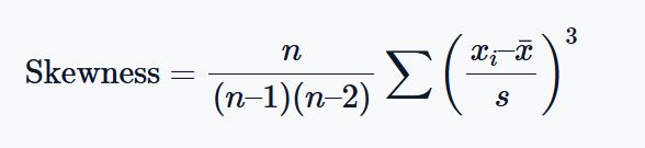
In real world scenario, you’re less likely to find yourself calculating skewness manually.
However, using the descriptive statistics calculator, the skewness of the sample data is 0.09.
This implies that the distribution of the data is almost symmetrical.
15. Kurtosis
Kurtosis is a statistical measure of the tailedness of a probability distribution. It describes the extent to which a dataset has outliers compared to a normal distribution. In other words, kurtosis quantifies whether the tails of the distribution are “heavy” (many outliers) or “light” (few outliers). A higher kurtosis indicates more outliers, often with a sharper peak, while a lower kurtosis indicates fewer outliers, typically with a flatter peak.
The kurtosis formula is:
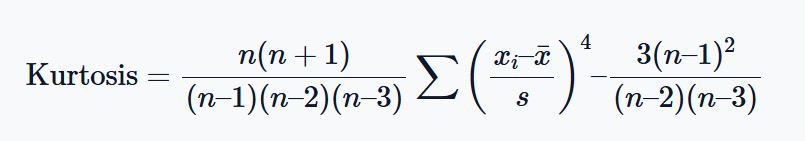
Similar to Skewness, you cannot be asked to compute kurtosis manually. However, using the calculator, the kurtosis for the sample data is approximately -1.64. This implies that the distribution is flatter than a normal curve (platykurtic).
Frequently Asked Questions
A Descriptive Statistics Calculator is a free online tool that helps you quickly compute key summary statistics like mean, median, mode, standard deviation, variance, range, and quartiles. It saves time by automatically handling the calculations you would normally do in Excel or by hand.
Descriptive statistics are used to summarize and describe the main features of a dataset. They help you understand the data’s central tendency, spread, and shape, making it easier to interpret patterns before doing deeper analysis or inferential statistics.
The calculator automatically ignores missing or non-numeric values. You can safely paste data directly from Excel or any text editor, and it will only process valid numeric entries.
Yes. The calculator allows you to select whether your data represents a sample or a population, and it automatically applies the correct formulas for variance and standard deviation.
It provides a complete summary including: count (n), mean, median, mode, minimum, maximum, quartiles (Q1 and Q3), interquartile range (IQR), range, variance, standard deviation, skewness, kurtosis, and outliers.
This calculator is fast, easy to use, and doesn’t require formulas or setup. You just paste your data and get instant results. It’s perfect for students, data analysts, and researchers who need quick descriptive statistics without complex tools.