Understanding the Binomial Distribution

The binomial distribution is a discrete probability distribution commonly used to model situations where an experiment is repeated a fixed number of times and each trial has only two possible outcomes (success or failure). The outcomes of a binomial experiment are either success or failure, yes or no, or pass or fail. Examples of binomial experiments include:

• Counting the number of heads when a coin is tossed several times
• Counting the number of defective items that appear in a batch
• Counting the number of respondents who answer “yes” in a survey.

To gain a comprehensive understanding of the binomial distribution, this article explains key binomial distribution concepts such as the formula, when to use a binomial distribution, key conditions for a binomial experiment, how to find binomial probability, mean and variance of a binomial experiment, and real-world applications of the binomial distribution.

When Should You Use the Binomial Distribution?

Wondering when to use a binomial distribution? You should use a binomial distribution only when your problem satisfies all the conditions of a binomial experiment. The four key conditions of a binomial experiment are:

1. The experiment has a fixed number of trials (n).
2. Each trial has only two possible outcomes (success or failure).
3. The probability of success (p) is the same for every trial.
4. The trials are independent of each other, and one outcome does not affect the other.

Binomial Distribution Formula

The binomial distribution formula allows us to compute the exact probability of getting x successes in n independent trials, provided the probability of success remains constant. The formula is:

P(X=x) =ⁿC_x . p^x . (1-p)^n-x

Where:

• n is the number of times the experiment is repeated
• x is the number of successes you want to compute
• p is the probability of success in a single trial
• 1-p is the probability of failure in a single trial
• ⁿC_x is read as “n combination x,” and represents the number of times you can get x successes in n independent trials.

You can directly compute ⁿC_x using a calculator or using the combination formula: ⁿC_x = n!/x!(n-x)!

Note. The probability of failure is often denoted using the letter q. Therefore, some books/articles will write the binomial probability formula as ⁿC_x . p^x . q^n-x

Solving Binomial Probabilities: Examples

To help you learn how to find binomial probability using the formula, follow these two examples.

Example 1

A fair coin is tossed 5 times. What is the probability of getting exactly 2 heads?

Solution

Since the coin is far, the probability of success, p = 0.5

The number of independent trials, n = 5

We need to find P(x=2)

To find P(X=2), we only need to apply the binomial probability formula.

Thus, P(X=2) = ⁵C₂ . 0.5² . (1-0.5)^5-2

= 10 * 0.25 * 0.5³

=0.3125

Therefore, the probability of getting exactly 2 heads in 5 coin tosses is 0.3125, or 31.25%.

Example 2

Peter guesses on all 10 questions of a multiple-choice quiz. Each question has 4 answer choices, and Peter needs to get at least 7 questions correct to pass. Compute the probability that Peter will pass the quiz.

Solution

Since there are 4 choices per question, the probability of success, p = 1/4 = 0.25

The number of independent trials, n = 10

We need to find P(X≥7). This is also called the cumulative probability of getting 7 or more correct answers.

Since the binomial distribution formula only allows us to compute exact probabilities, we need to apply that discrete probability to solve the problem.

Thus, P(X≥7) = P(x =7) + P(x=8) + P(x=9) + P(x=10)

This means we need to compute each of the exact probabilities above and sum them to get the results.

P(x=7) = ¹⁰C₇ . 0.25⁷ . (1-0.25)^10-7

=120 * 0.000061 *0.421875

=0.00309

P(x=8) = ¹⁰C₈ . 0.25⁸ . (1-0.25)^10-8

=45 * 0.0000153* 0.5625

=0.000386

P(x=9) = ¹⁰C₉ . 0.25⁹ . (1-0.25)^10-9

=10 * 0.25⁹ * 0.75¹

=0.0000286

P(x=10) = ¹⁰C₁₀ . 0.25¹⁰ . (1-0.25)^10-10

=1 * 0.25¹⁰ * 1

=0.000000953

Thus, P(X≥7) = 0.00309 + 0.000386 + 0.0000286 + 0.000000953

=0.0035

Therefore, the probability that Peter passes the quiz by guessing alone is approximately 0.0035, or 0.35%. This means that it was very unlikely to pass the test with random guessing.

Want more examples? Check out our complete guide on how to calculate binomial probability

However, if you know how to identify the parameters, n, p, and x from a binomial probability question, and want a quicker way to get binomial probabilities, try the binomial distribution calculator. This calculator helps you find the exact and cumulative probability of any x.

Mean and Variance of a Binomial Distribution

The mean and variance of a binomial distribution describe its center and spread. They help us summarize what outcomes you should expect on average and how much variability there is around that average when a binomial experiment is repeated many times.

The mean/expected value of the binomial distribution is μ = np.

Where:

• n is the number of trials
• p is the probability of success

It represents the average number of successes you would expect if you were to repeat the experiment n times.

Example 1. Find the mean of a binomial experiment with 20 trials, given that the probability of success is 0.3

From the question, n = 20 and p = 0.3

Therefore, we can compute the mean as follows:

μ=n × p

= 20 × 0.3

= 6

The variance of the binomial distribution is σ² = npq or σ² = np(1-p).

Where:

• n is the number of trials
• p is the probability of success
• q = 1- p and represents the probability of failure

It measures how much the number of successes tends to vary around the mean. A larger variance indicates more spread in the possible outcomes.

Since the standard deviation is the square root of the variance, you only need to find the square root of the variance of a binomial distribution to get its standard deviation.

Example 2. Find the variance and standard deviation of a binomial experiment with 20 trials, given that the probability of success is 0.3

By definition, variance, σ² = np(1-p).

= 20 * 0.3 (1-0.3)

= 4.2

To find the standard deviation, you simply find the square root of 4.2, which gives 2.05

Shape of the Binomial Distribution

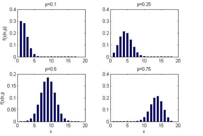
The shape of a binomial distribution varies by the number of trials (n) and the probability of success (p). When the number of trials is small, the distribution appears more discrete and uneven. However, as n increases, the distribution becomes smoother and begins to resemble a continuous curve.

The value of p determines whether the distribution is symmetric or skewed. Here’s how you can master the shape of the binomial distribution:

• When p = 0.5, the distribution is symmetric around the mean.
• When p< 0.5, the distribution is skewed to the right
• When p>0.5, it is skewed to the left.

The figure below shows the shape of the binomial distribution as you increase the probability of success, p.

Normal Approximation to Binomial

While it is easy to find binomial probabilities using the formula, the process can become complex as the number of trials increases. In this case, you need to apply a concept known as the normal approximation to the binomial. This concept is derived from the idea that when the number of trials is sufficiently large, the shape of the binomial distribution becomes smooth and symmetric.

Note. You should only apply the normal approximation to a binomial if the following conditions are met:

• np ≥ 5
• n(1−p) ≥ 5

The normal approximation is useful because it simplifies probability calculations for large sample sizes, where direct binomial computation can be tedious.

Want to learn more about this concept? Check out the guide to the normal approximation to the binomial.

Practical Applications of the Binomial Distribution

The binomial distribution is widely used in solving many real-world problems. Here are just but a few examples:

Monitoring Processes and Decision Thresholds

The binomial distribution is widely used in quality control to determine whether the results fall within the expected limits. For example, when items are sampled from a production run, the distribution is used to estimate how unusual a given number of failures or defects is. This helps managers decide whether the performance of the process is normal or needs to be improved.

Analyzing Binary Responses in Data Collection

Many real-world datasets consist of binary outcomes, such as approval versus rejection or presence versus absence of a trait. The binomial distribution provides a framework for analyzing how many observations fall into one category. This is especially useful in survey analysis and experimental research.

Modeling Uncertainty in Predictive Scenarios

The binomial distribution is also used to model uncertainty in scenarios where outcomes unfold step by step. By assigning probabilities to success and failure at each step, analysts can evaluate different outcome paths and their likelihoods.

Frequently Asked Questions