Descriptive statistics are methods or techniques that are widely used to organize and summarize data in a clear and simple way. In data analysis, descriptive statistics serve as preliminary tests to help you organize, summarize, and uncover the main characteristics of the data. Simply stated, these statistics allow you to gain an overview of the data before diving into the deeper analysis. In real-world situations, they can help you uncover hidden insights into the data such as errors, unusual values, and general trends. Thus, this article will teach you what descriptive statistics are, their different types, and how to calculate key statistics using practical examples.
What Are Descriptive Statistics?
Definition: Descriptive statistics are methods used to summarize and decribe the main features of a dataset. These statistics are useful because they help you gain a brief overview of the distribution of the data. Thus, the main aim of descriptive statistics is to give you a quick and accurate overview of your data before doing any advanced analysis.
Descriptive statistics are different from inferential statistics. While descriptive statistics only describe what is already in the dataset, inferential statistics use sample data to make inferences about the target population. This means that unlike inferential statistics which rely on sample data, descriptive statistics can be calculated for both sample and population data to help you explore the data, check for errors, identify hidden insights/trends, or even present the data using simple summaries.
Types of Descriptive Statistics
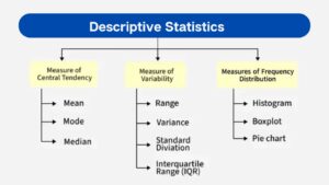
To fully understand descriptive statistics, it is important to be familiar with its different types. Knowing these types provides a foundation for analyzing and interpreting data effectively. The three main types of descriptive statistics include:
- Measures of Central Tendency
- Measures of Dispersion
- Measures of Frequency Distribution
In addition to these three primary categories, some studies also recognize a fourth type, known as measures of position. Each of these measures, along with practical examples is presented below:
1. Measures of Central Tendency
The measures of central tendency are the summary statistics that attempts to describe a whole set of data using a single value representing the middle or center of its distribution. They can inform you where the most numbers in the data fall. The three main measures of central tendency are:
- Mean
- Mode
- Median
Mean
The mean is the arithmetic average of all values. You can find the mean of any dataset by summing all the values and dividing by the number of observations. Thus, the mean formula is:
Mean = ΣX/N
Where:
- ∑X is the sum of all values
- N is the total number of observations.
Example. A manager wants to know the average number of units sold per day over 5 days. The unit sold for the five days were: 12, 15, 10, 18, 15.
To find the mean of the data, follow these steps:
- Sum all the values. We have 12+15 +10+18+15 = 70
- Count the total number of observations. In this case, we only have 5 observations.
- Compute the mean. By definition, mean = ΣX/N = 70/5 = 14
Thus, the average number of units solds per day was 14.
Want an easy way to calculate the sample mean? check out our free sample mean calculator to get instant and accurate results.
Median
The median is the middle value when the data is arranged in order. This means, to find the median of a dataset, you need to first arrange the data either in ascending or descending order and then find the values that lies in the middle. Simply stated, you can calculate the median of any dataset by following these simple steps:
- Arrange the observations either from smallest to largest (ascending order) or from largest to smallest (descending order).
- If the number of observations is odd, the median is the middle value.
- However, if the number of observations is even, the median is the average of the two middle values.
Example. A real estate agent wants to know the typical house price. The collected data was as follows:
Data (in $000): 120, 150, 300, 160, 155
To calculate the median, we follow these steps:
- Arrange the data in ascending order: 120, 150, 155, 160, 300
- Since the number of observations is even (n = 5), then the median is the middle value. Thus, median = 155.
Note. The median gives a better picture than the mean because house prices often include extreme values.
Mode
The mode is the value that appears most often in any dataset. There is no formal formula for finding the mode. However, the rule of hand is to identify the value with the highest frequency in the dataset.
Example. A shoe store wants to know the most common shoe size purchased in a week. The shoe sizes that were bought in the week were: 7, 8, 8, 9, 7, 8, 10, 9.
To find the mode, you can easily identify the most repeated shoe size in the data. In this case, the most repeated number is 8 (repeated 3 times). Thus, Mode = 8. In other words, the most common shoe size purchase in a week is 8.
Note. A dataset can have more than one mode:
- If there are two modes, the data is called bimodal.
- If there are three modes, it is called trimodal.
- If there are more than three modes, it is referred to as multimodal.
Key Tips about Measures of Central Tendency
- The mean works well for clean, balanced data.
- The median is best for skewed data or values with outliers.
- The mode is ideal for understanding the most common category or repeated number.
2. Measures of Dispersion (Variability)
Measures of dispersion/variability show how spread out the values in a dataset are. They help you understand whether the data is tightly packed or widely scattered. The main measures of dispersion are:
- Range
- Interquartile range (IQR)
- Variance
- Standard Deviation
Range
The range is the difference between the largest and smallest values. Thus, to find the range of any dataset, you need to subtract the smallest value from the largest value. Thus, the range formula is:
Range = Maximum – Minimum
Example. A teacher wants to see how much test scores vary in a class. Given the data: 50, 65, 70, 80, 90, calculate the range.
By definition, Range = Maximum – Minimum
=90-50
= 40
A range of 40 shows the scores vary widely.
Interquartile Range (IQR)
The Interquartile Range (IQR) measures the spread of the middle 50% of the data. It is less affected by extreme values. The IQR formula is:
IQR = Q3 – Q1
Where:
- Q1 is the lower quartile
- Q3 is the upper quartile
Example. A company wants to compare the typical monthly expenses of employees. The expenses for five employees are as follows: 800, 1000, 1200, 1500, 1800.
To calculate the Interquartile range, we follow these steps:
- Sort the data from least to greatest
- Find the median of the entire dataset to divide it into a lower and upper half
- Find the median of the lower half to get Q1
- Find the median of the upper half to get Q3
- Calculate the IQR using the formula: IQR = Q3-Q1
Following the steps, Q1 = 1000 and Q3 = 1500.
Thus, IQR = 1500-1000
= 500
This means the central half of expenses ranges across 500 units.
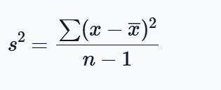
Variance
Variance is a measure of dispersion which shows how far values are spread out from the mean. You can easily calculate the sample variance using the formula:
Example. A fitness coach tracks daily steps for 5 days are: 8000, 9000, 7000, 10000, 9000. Calculate the variance.
To calculate the variance, we need to apply the variance formula. As you’ll note, we will need the sample mean, x̄ to calculate the deviation of each data value from the mean.
By definition, sample mean, x̄ = Σx/n
= (8000+ 9000 + 7000+ 10000+ 9000)/5
= 43000/5
=8600
Let’s use a table to to find the sum of deviations from the mean, Σ(xi-x̄ )
| x | (xi-x̄)^2 |
|---|---|
| 8000 | (8000-8600)^2 =360,000 |
| 9000 | (9000-8600)^2 = 160,000 |
| 7000 | (7000-8600)^2 = 2,560,000 |
| 10000 | (10000-8600)^2 = 1,960,000 |
| 9000 | (9000-8600)^2 = 160,000 |
Thus, Σ(xi-x̄ )^2 = (360,000 + 160,000 + 2,560,000 + 1,960,000 +160,000)
=5,200,000
Thus, the sample variance, S^2 = 5,200,000/(5-1)
= 1,300,000
Standard Deviation
Standard deviation is the square root of the variance. It tells you how far, on average, each value is from the mean. Thus, given that the variance of the above data is 1,300,000, you can easily compute the standard deviation by taking the square root of the variance.
Hence, standard deviation = sqrt (1,300,000)
=1140.18
This means daily steps typically differ from the mean by about 1140.18 steps.
3. Measures of Frequency Distributions
A frequency distribution is a way to summarize and organize data to show how values are spread across categories or intervals. It helps you see patterns, identify outliers, and understand the overall structure of the dataset. Frequency distributions are often the first step in analyzing data before applying more advanced methods or creating visualizations like histograms, bar charts, or pie charts.
A frequency distribution table usually includes:
- Data intervals or categories – the values or groups being measured
- Frequency counts – how many times each value or group occurs
- Relative frequencies – percentages showing the proportion of each category
- Cumulative frequencies – totals up to a certain value, useful for calculating medians or percentiles
Frequency distributions make large datasets easier to understand. They help you identify trends, the most common values, and unusual data points. They also provide the foundation for graphs and charts. This consequently makes data more visual and easier to interpret for reports, research, or business decisions.
4. Measures of Position
Measures of position show where a specific value lies within a dataset. They help you understand how a value compares to the rest of the data. The main measures of positions include percentiles, quartiles, and z-scores. These measures are commonly used in education, health, finance, and many other fields.
Percentiles
Percentiles divide data into 100 equal parts. As such, each percentile tells you the percentage of values that fall below a certain point. For instance, if a score is at the 70th percentile, then it means that it is higher than 70% of all scores.
Quartiles
A quartile is one of three values that divide a sorted data set into four equal parts. The three quartiles are:
- The first quartile (Q1), which is also known as the 25th percentile. This means that 25% of the data falls below this value. In other words, it is the median of the lower half of the data.
- The second quartile (Q2), which is the median or 50th percentile. It divides the data into two equal halves.
- The third quartile (Q3), which is also called the 75th percentile. This means that 75% of the data falls below this value. Simply stated, it is the median of the upper half of the data.
Z-Scores
A z-score shows how many standard deviations a value is from the mean. It is calculated using the formula: z = (x-μ)/σ. They are widely used to standardize raw scores into z values in the normal distribution.
Want to learn more about how to calculate z scores manually and using a calculator? Check out our z-score calculator with steps.
Table 1: Summary of the Types of Descriptive Statistics
| Type of Descriptive Statistic | What It Measures | Common Measures | Purpose / What It Tells You |
|---|---|---|---|
| Measures of Central Tendency | The center or typical value of a dataset | Mean, Median, Mode | Shows the average or most representative value in the data |
| Measures of Dispersion (Variability) | The spread or variation in the dataset | Range, Variance, Standard Deviation, Interquartile Range (IQR) | Indicates how much the data points differ from each other and from the center |
| Measures of Frequency Distribution | How often values occur within categories or intervals | Frequency tables, Percentages, Histograms | Helps identify patterns, trends, and the distribution of data |
| Measures of Position | The relative standing of a value within a dataset | Percentiles, Quartiles, Z-scores | Shows the position of a score compared to the rest of the dataset |
Key Takeaways
- Descriptive statistics help simplify and summarize large datasets into understandable insights.
- Measures of central tendency show the “middle” or typical value in a dataset.
- Measures of dispersion reveal how spread out or varied the data is.
- Frequency distributions help you identify patterns and how often values occur.
- Measures of position allow you to compare individual scores to the rest of the dataset.
- Understanding these measures gives you a strong foundation for more advanced statistical analysis.
Ready to Put These Concepts Into Practice? Try our Descriptive Statistics Calculator to instantly compute measures like mean, median, mode, range, variance, and standard deviation. It’s fast, accurate, and perfect for students, researchers, and professionals who want quick insights from their data.
Frequently Asked Questions
Descriptive statistics refers to methods used to summarize and organize data. It helps you understand the basic features of a dataset by describing its central values, spread, and overall pattern.
The four commonly recognized types are:
– Measures of central tendency
– Measures of dispersion
– Measures of frequency distribution
– Measures of position
Descriptive statistics summarize what the data shows. Inferential statistics go a step further and use sample data to make predictions or draw conclusions about a larger population.
The main purpose of descriptive statistics is to present data in a clear and meaningful way. It helps you understand what the data shows by summarizing key features such as averages, variability, and patterns.