F Critical Value in Excel

After performing an F-test for ANOVA, equality of variance test, or a regression model, you obtain an F-test statistic. The next step involves finding an F-critical value to help you determine whether the results are statistically significant or not. There are various methods for finding F-critical values. The classical approach involves reading critical values from f-tables. However, for quick and accurate solutions, an online f-critical value calculator or Excel function can be very helpful. In this article, you’ll learn how to find the f critical value using the Excel function (with worked out example).

How to Find the F Critical Value in Excel

To find the F-critical value in Excel, we use the F.INV.RT() function. The function accepts three key parameters, which include:

• Significance level, α
• The numerator degrees of freedom, df1
• The denominator degrees of freedom, df2

With the three parameters, you can easily find the F critical value using the formula =F.INV.RT(α, df1, df2). Therefore, to find the critical F value using Excel, follow these steps:

1. Open a blank Excel sheet
2. In a cell where you want the F-critical value to appear, type the formula =F.INV.RT(alpha, df1, df2). (You should replace alpha, df1, and df2 with your actual values)
3. Press the Enter key.

Excel will instantly return the correct critical value for your F test.

Finding the F-Critical Value Using Excel: Example

Imagine you want to compare the variance of two production lines in a factory. You plan to run an F-test to see if the variability in output is different between the two lines. Assuming a 5% significance level, 4 numerator degrees of freedom, and 10 denominator degrees of freedom, find the appropriate F critical value for this test.

Solution

From the scenario, we can identify the three parameters as follows:

• Significance level, α = 5% = 0.05
• The numerator degrees of freedom are 4
• The denominator degrees of freedom are 10

Therefore, to find the F-critical value for the test using the F.INV.RT() function, follow these steps:

• Step 1: Open a Blank Excel sheet
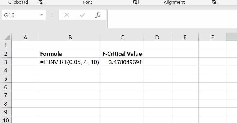
• Step 2: In a cell where you want the critical value to appear, type the formula: =F.INV.RT(0.05, 4, 10)
• Step 3: Press the Enter key

The Excel formula will return the correct critical value for the test as 3.4780 (see Figure 1).

Note. You can also confirm the value using the F distribution table. In this case, you need to look up the f-table with alpha = 0.05 and look for the intersection of df1 = 4 and df2 = 10.

Quick Tips

Here are a few tips to keep in mind to avoid mistakes when calculating critical F values in Excel:

1. Double-check your degrees of freedom. Make sure the numerator (df1) and denominator (df2) are correct. Reversing them will give the wrong value.
2. Use the correct significance level. Common choices are 0.01, 0.05, or 0.10. Enter it as a decimal, like 0.05.
3. Always use F.INV.RT. This function gives the right-tail F-critical value. Avoid using older functions like FDIST unless you are using legacy Excel versions.
4. Ensure no extra spaces or errors in the formula. Even small mistakes in typing the formula can cause errors.
5. Compare carefully. Remember, the F-statistic must be greater than the F-critical value to reject the null hypothesis.